Geo-spatial Data & Site Characterisation

Geo-spatial Data and Site Characterisation

The first benefit of investigation is not increased confidence, but removal of false confidence.

This page sets out Albian-Geo’s technical approach to geo-spatial data and site characterisation: how observations are collected, positioned, attributed, analysed and communicated so that they become defensible information rather than misleading maps or overconfident models.

Geo-spatial data underpins almost every investigation of the subsurface or near-surface environment.

Collected from boreholes, trial pits, geophysical surveys, remote sensing, or surface sampling, such data begins its life as a set of numbers tied to positions in space.

Sample and micro-scale analyses are important, but their value depends on interpretation within the wider site characterisation model.

Individual results describe specific materials or locations; site understanding comes from linking those results to spatial distribution, geological setting, groundwater conditions, historical land use, and the processes controlling variability across the project area.

The journey from raw dataset to defensible site understanding — one that can withstand technical scrutiny, inform risk assessment, and support engineering or environmental decisions — is neither automatic nor guaranteed.

Geo-spatial data is collected and transformed into information...

Geo-spatial information is attributed, organised and interrogated...

This information, properly presented allows the visualisation and comprehension of complex 3D and temporal situations.

For Geo-spatial data to provide meaningful information or insights it must be:

Observed
Preserved
Processed
Analysed
Communicated

Not all geo-spatial data is created equally. Reliability of geo-spatial data is therefore dependent upon:

The quality of the sampling.
The quality of the position.
The quality of the data attribution.
The relevance of the data.

Note: In order to visualise and measure your geo-spatial data within the wider context of the project domain, it is imperative to accurately position it in the correct coordinate reference system.

For site characterisation, the key questions are:

What is the purpose and objectives of the investigation?
Is the apparent pattern real, or an artefact of sparse or biased sampling?
Does the variability reflect a known geological, hydrogeological, geomorphological or land-use control?
Are there distinct spatial domains that should be interpreted separately?
Is the sample spacing appropriate for the scale of variability being mapped?
Are sufficient samples collected to provide meaningful analysis?
Are predictions being made by interpolation between reliable observations, or by extrapolation beyond the area of data control?

Assumptions About Your Data

Everything is related to everything, but near things are more related. (Tobler 1970)

But....

Your data is rarely collected with the aim of providing good spatial statistics for the geo-statistician…

Budgetary constraints
Minimum required (for representative sample)
Scale of observations/measurements
Targeted with bias

It is also likely that you may be relying on 3rd party data

Errors WILL propagate throughout the computational, analytical process.

Unless your data:

Have been collected, analysed or measured in a fit and proper manner.
Have been pre-screened to identify blunders and outliers; you should consider:
- Different sampling campaigns
- Consistent sampling procedures
  - Signs: Differences in reporting precision, sample numbering, missing samples
- Have positions been verified (plot on a map).

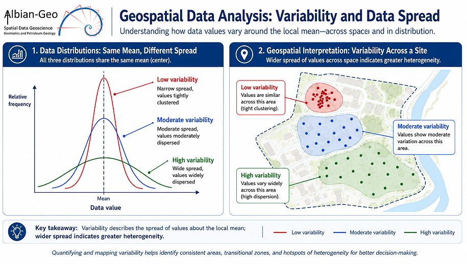
Site Characterisation and its Variability

Site characterisation depends on understanding both the local mean and the spread of values around that mean.

Where values are consistent, interpolation between reliable observations may provide a reasonable basis for prediction. Where values are highly variable, a single observation may not represent the surrounding area, and local estimates become less certain.

In practical terms, high variability may indicate changes in geology, made ground, groundwater conditions, contamination, drainage pathways, or historical land use. It may also reflect sampling bias, poor spatial coverage or measurement uncertainty.

This affects all spatial estimation methods, including contouring, gridding, interpolation, kriging and 3D ground modelling.

A visually smooth map is not necessarily a reliable model. The interpretation must be supported by data quality, sampling density, spatial coverage and a defensible conceptual site model.

The aim is therefore not simply to produce a map, but to identify where the data support reliable interpolation, where uncertainty remains high, and where further targeted investigation is needed.

Site Characterisation:
How many samples are needed?

There is no single formula that defines the correct number of samples for spatial site characterisation.

Simple statistical sample-size formulae based on confidence level and margin of error can be useful for estimating a general population mean or proportion. However, they are not, on their own, suitable for designing a spatial investigation.

In geospatial work, the value of a sample depends on both what is measured and where it is measured. Sample number must therefore be considered together with sample spacing, spatial coverage, site heterogeneity, depth, data quality, measurement uncertainty and the conceptual site model.

The required sampling density depends on the scale of variability being investigated. If site conditions change gradually over distance, fewer well-positioned samples may support reasonable interpolation.

If conditions change over short distances, more closely spaced samples may be required.

A defensible sampling design should consider:

the purpose of the investigation;
the parameter being measured;
the expected scale of spatial variability;
the size and geometry of the site;
whether the site contains different geological, hydrogeological or land-use domains;
whether the aim is to estimate an average value, detect a hotspot, define a boundary, or support interpolation;
the acceptable consequence of missing an important feature;
whether sampling is random, grid-based, stratified, targeted, transect-based or adaptive;
the need for validation or check samples;
the cost of additional samples compared with the cost of uncertainty.

For spatial data, the question is therefore not simply “How many samples are needed?”. A better question is:

How many samples are needed, where should they be located, and at what spacing, to characterise the variability relevant to the decision being made?

Each sample will also have a cost impact

Collection, analysis complexity, time, errors
Avoid unnecessary samples - waste of resources

Basic Analysis:
Univariate and Bivariate

Univariate Analysis

Provides a first statistical description of each parameter.
Identifies the central tendency: mean, median and typical value.
Quantifies spread: range, standard deviation, percentiles and outliers.
Highlights skewed, mixed or multi-modal populations.
Helps decide whether a single site-wide summary is meaningful.
Supports early screening of anomalous results and possible data errors.
Does not, on its own, explain where values occur spatially.

Bivariate analysis

Bivariate analysis considers the relationship between two variables.

It answers questions such as:

Do two parameters increase or decrease together?
Is the relationship linear, non-linear or absent?
Is one variable potentially acting as a proxy for another?
Are different populations being mixed together?
Are there threshold effects or domain-specific trends?
Do outliers control the apparent relationship?
Does the relationship make geological, hydrogeological or environmental sense?

Bivariate analysis can be powerful, but it requires caution.

A good correlation may reflect a real process, but it may also be caused by sampling bias, shared spatial trend, common depth control, mixed populations, or an unrecognised third variable. Correlation should therefore be interpreted against the conceptual site model, not treated as proof of causation

Residuals and model checking

A regression line is not sufficient on its own. The residuals — the differences between observed and predicted values — should be reviewed to determine whether the relationship is valid.

Residual analysis is an important check on bivariate and regression models. If the residuals show a systematic pattern, then the model has not fully explained the structure in the data. In site characterisation, patterned residuals may indicate separate geological domains, spatial autocorrelation, sampling bias, depth effects, groundwater controls or an unrecognised process influencing the dataset.

Autocorrelation

Autocorrelation in spatial data refers to the correlation of a variable with itself through space. It describes how similar data values are based on the distance and direction between them.

Why it is important:

Identify clustering, gradients, or randomness in spatial distributions
Strong positive autocorrelation implies nearby data points are good predictors for unknown values — a core idea behind kriging and contouring.

If autocorrelation is unexpectedly high or low, it may point to issues like:
- Measurement bias
- Systematic environmental variation
- Over-sampling (duplicate or near-duplicate points)

Model Assumptions
Many statistical models assume observations are independent. Spatial autocorrelation violates this — meaning traditional stats (like regression) may give misleading results.

Before spatial interpolation, contouring, kriging or 3D modelling are undertaken, the dataset should be understood statistically.

Basic statistical analysis helps identify the character of the data, the presence of outliers, the likely controls on variability, and whether relationships between variables are meaningful or misleading.

Univariate and bivariate analysis are simple methods, but they are important quality-control steps.

They help determine whether the dataset is suitable for mapping, whether it should be separated into different spatial or geological domains, and whether apparent trends are real or caused by sampling bias, mixed populations or measurement uncertainty.

Site Characterisation:
Displaying and Prediction of the Results

Displaying and Prediction of Results P.png

How good are your maps or results

A helpful qualitative display with questionable quantitative significance’ Isaacks (1989)

Maps, contours, grids and 3D models are useful ways to communicate spatial data, but a visually smooth output is not necessarily a reliable prediction.

The quality of the result depends on the input data, sample spacing, spatial coverage, sampling bias, variability, interpolation method and the conceptual site model.
Different contouring methods can produce different surfaces from the same dataset, so the method and its assumptions should be stated clearly.
Prediction is strongest where values are interpolated between reliable observations.
Confidence reduces where data are sparse, clustered, highly variable or where results are extrapolated beyond the area of data control.
Anomalies should be checked before interpretation.
They may represent real geological, hydrogeological or environmental features, but they may also be caused by positional error, sampling bias, analytical error, edge effects or processing artefacts.
A defensible spatial output should therefore show the predicted result together with the data control, interpolation limits, validation/check points and areas of uncertainty.

Key considerations about the mapped results

A map is a model, not the ground truth.
Smooth contours can create false confidence.
Different interpolation methods can produce different results from the same data.
Sample location and spacing may be more important than sample number alone.
Clustered samples can bias the apparent spatial pattern.
Predictions are strongest where supported by surrounding data.
Extrapolation beyond data control should be clearly identified.
Calibration or validation points should be used where possible.
Anomalies may be real features or processing artefacts.
Interpretation should be consistent with the conceptual site model.
Maps should show data points, not only the interpolated surface.
Uncertainty should be communicated, not hidden.

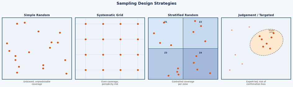
Sampling Design Strategy

Beyond the question of how many samples, the pattern in which they are collected matters enormously for the statistical validity of subsequent analysis.

Four principal strategies are in common use

Strategy - Characteristics and Trade-offs

Simple Random

Each location is selected independently with equal probability. Unbiased but can produce uneven coverage, particularly in small samples. Valid for classical statistical inference.

Systematic Grid

Samples placed at regular intervals across the site. Ensures even spatial coverage and is efficient for interpolation, but is vulnerable to periodicity effects if the site has regular structure at the same spacing.

Stratified Random

The site is divided into zones based on prior knowledge — geology, land use, contamination risk — and random samples are drawn within each zone. Balances statistical validity with targeted coverage.

Judgement / Targeted

Samples placed based on expert knowledge of likely hotspots or features of interest. Efficient for finding anomalies but introduces spatial bias and limits the validity of site-wide statistical inference.

Judgement sampling is not inherently wrong — it is often the right choice for targeted investigation.

However, results from a judgement sample cannot be legitimately extended to the wider site using standard statistical methods without acknowledging the bias.

The sampling strategy must match the analytical intent.

Geo-hazards and Made Ground

Geo-hazards are not treated as isolated map features, but as part of the wider site conceptual model, linking geology, geomorphology, groundwater, surface processes, land use and project vulnerability. Some geo-hazards are:

Flooding and floodplain constraints
Erosion and scour
Slope instability and landslide potential
Soft ground and differential settlement risk
Buried channels and ground variability
Subsidence and ground collapse
Coastal change and shoreline instability
Shallow groundwater constraints
Contaminant migration pathways
Liquefaction susceptibility

Made ground and landfill-affected sites can introduce complex geohazards, including variable ground conditions, settlement risk, contamination, ground gas migration, and leachate breakout.

Methane, carbon dioxide, and contaminated leachate may move through permeable strata, service trenches, fractures, or other preferential pathways, potentially affecting foundations, buildings, groundwater, surface water, and buried infrastructure.

Robust site characterisation is therefore essential to define the extent and behaviour of made ground, identify gas and leachate migration pathways, and support appropriate engineering, environmental, and monitoring measures.

GIS, historical mapping, remote sensing, field observations and intrusive investigation can be combined to identify former structures, infilled areas, spoil, waste deposits, buried obstructions and zones of possible contamination or settlement risk.

Historical Maps, Drawings and Land Changes

Historical maps, aerial photographs, satellite imagery and project records can show how a site has changed through time.

Former land use, drainage modification, excavation, infilling, industrial activity, flooding, erosion, construction and demolition can all leave ground conditions that are not obvious from current site inspection alone

Integration of historic records into GIS to compare past site conditions with present-day topography, infrastructure, land use, groundwater conditions and proposed development layouts.
Identification of data gaps, inconsistencies and conflicts between historic records, modern imagery, field observations and current project datasets.
Recognition that historic data can be highly valuable, but should not be accepted uncritically; old records require validation against current survey control, field evidence and modern investigation data.

Geotechnical and Geophysical Subsurface Characterisation

Geotechnical and geophysical understanding are important parts of site characterisation because they help define how the ground varies beneath a site, not just what has been observed at individual investigation points.

Ground strength, compressibility, groundwater conditions, made ground, buried channels, variable rockhead, weak strata and obstructions can all affect foundations, roads, earthworks, excavations, retaining structures, drainage, pipelines and long-term settlement performance.

Geotechnical appraisal is particularly important where the proposed development includes:

Buildings, tanks, foundations or other load-bearing structures
Roads, pavements, working platforms and hardstanding areas
Embankments, land-raising, cuttings or engineered fill
Excavations, retaining walls, basements or temporary works
Pipelines, buried services, drainage systems and utility corridors
Coastal, river, alluvial, reclaimed or low-lying ground
Areas of made ground, landfill, soft soils, loose granular deposits or shallow groundwater
Slopes, erosion-prone ground, buried channels or variable rockhead
Sites affected by previous industrial, construction, demolition or earthworks activity

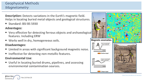
Geophysical methods can add significant value where intrusive investigation alone cannot practically define the scale and continuity of subsurface variation. They may help identify changes in ground conditions between boreholes, possible buried features, infilled ground, shallow rockhead, voids, services, groundwater-related contrasts or zones requiring further targeted investigation.

However, geophysical results should not be treated as standalone answers. They require calibration against boreholes, trial pits, sampling, testing, geological interpretation and site history.

The value of geotechnical and geophysical information lies in how it contributes to the wider site conceptual model. Individual test results, investigation records or geophysical anomalies should be used to define ground domains, identify spatial variability and constrain interpretation between reliable observations.

Data should be interpreted primarily by interpolation between supported investigation points.

Extrapolation beyond the area of investigation should be treated with caution, because it can create false confidence and produce ground models that appear precise but are not properly constrained by evidence.

A reliable interpretation should therefore integrate geotechnical data, geophysics, geology, geomorphology, groundwater, contamination, historical land use, spatial data quality and proposed development constraints, so that ground-related risks can be identified early and managed appropriately.

Geo-spatial Data
A Project Schema & Geo-spatial Uncertainty Curve

Geospatial projects often exist in complex 3D environments both at, and beneath the ground surface.

From project conception through to execution and eventual completion, Geo-spatial data and its transformation to credible information is poorly understood and is an often side-lined facet of the project.

Because many projects begin with unjustified certainty - the first benefit of investigation is not increased confidence, but removal of false confidence.

For successful outcomes good quality geo-spatial data will reduce uncertainty, dispel incorrect pre-conceptions and add value to projects that require this data as a key foundation element:

Knowledge gaps are identified and rectified through a single data measurement or series of data measurements.
This data is organised and attributed, and transformed into information
This information yields insights from which informed decisions based on spatial knowledge can be made...
Reducing overrun and cost consuming changes to plan that were originally made on false pre-conceptions

Acknowledgement is made to Pyrcz, Isaaks, Deutsch, Smith and others from whom many of the above themes are based

A conceptual look at knowledge gained in an investigation

The idea is to treat the curve as a knowledge-gain function, where:

x = investigative input, effort, time, cost, or integrated investigation intensity
y = usable spatial knowledge, or defensible confidence in site understanding

Then: dy/dx Is the marginal knowledge gain per unit investigative effort.

Interpretation by project stage

Early stage: low dy/dx

Desk study, initial assumptions, rough conceptual model.
At this stage, effort may not immediately produce much reliable spatial knowledge. Some effort is spent identifying what is not known. There may even be confusion reduction rather than true knowledge expansion.
This is an important point: early effort is still valuable, but the apparent rate of gain in defensible knowledge may be small.

Transitional stage: increasing dy/dx

Knowledge gaps are identified, investigation becomes targeted, measurements begin to answer the right questions.
This is where each added unit of effort may yield large reductions in uncertainty. This is often the most efficient part of the investigation.

Mature stage: peak dy/dx

The investigation is well-designed, the main controls on variability are understood, and data are being transformed into robust spatial interpretation.
This is the zone of maximum return on investigative effort.

Late stage: declining dy/dx

Additional sampling, modelling refinement, and monitoring still help, but each new increment contributes less than before.
This is the diminishing-returns zone

A useful alternative perspective is that dy/dx does not merely depend on effort quantity. It depends on effort quality. So more rigorously dy/dx

is high when investigation is:

Correctly targeted
Spatially representative
Well-attributed
Properly analysed
Linked to the governing uncertainties

and low when effort is:

Ad hoc
Biased
Redundant
Poorly located
Not tied to the key conceptual uncertainties

This is probably the most important insight. The derivative is not just “how much work is being done,” but “how much useful understanding is being extracted from that work.”

The second Derivative

A further useful idea is the second derivative d2y/dx2

This indicates whether the rate of knowledge gain is accelerating or decelerating.

Conceptually:

d2y/dx2 > 0: investigation is becoming more effective, often because the conceptual model is improving and sampling is becoming better targeted
d2y/dx2 = 0: point of maximum efficiency growth, often near the inflection region
d2y/dx2 < 0: diminishing returns have begun

This can be very helpful if the aim is to argue for targeted investigation design rather than simply more investigation.

Area under the curve

The Spatial Certainty Curve can be viewed as a cumulative expression of spatial knowledge developed through investigation. Its gradient, dy/dx, represents the rate at which useful knowledge is gained as investigative effort increases.

The area under this rate curve represents the cumulative increase in spatial knowledge over a given range of effort, rather than the total possible knowledge.

Where spatial knowledge is expressed qualitatively rather than as a measured index, this relationship should be understood as a conceptual guide rather than a strict mathematical quantity.

Important caution

A common assumption would be that knowledge always increases smoothly with effort. In reality that is not always true.

Sometimes there may be temporary negative effects in perceived confidence:

Early investigation may reveal that prior assumptions were wrong
Confidence may drop before reliable knowledge rises
The curve may therefore include a “false confidence collapse” before the main rise

This is actually a very valuable idea for site investigation, because many projects begin with unjustified certainty. In those cases the first benefit of investigation is not increased confidence, but removal of false confidence.

So in a more realistic conceptual model:

Apparent confidence may fall first
Defensible knowledge then rises
Later gains diminish

When does a site investigation model move from conceptual to data driven?

In site characterization, the transition is not a single point, but a change in the basis of inference.

Practical distinction

A site understanding is mainly conceptual when interpretation is driven primarily by:

process knowledge,
geological or geomorphological reasoning,
analogue sites,
expert judgement,
sparse observations fitted into a plausible model.

A site understanding becomes more statistical or data-driven when the dominant conclusions are supported by:

a dataset with enough coverage to estimate variability,
reproducible summaries of central tendency and spread,
quantified spatial structure,
uncertainty estimates based on observations rather than assumption alone.

Ten high-quality observations do not create a statistical site model if the site varies at a scale smaller than the sample spacing.

So the threshold depends on the ratio between: sampling density and heterogeneity scale

A defensible threshold

A practical threshold is reached when three things are available together:

Requirement

Sufficient sample count
Sufficient spatial coverage
Quantified uncertainty

Why it matters

Needed to estimate distributions
Needed to detect structure, not just values
Needed for defensible inference

If one of these is missing, the understanding remains partly conceptual.

For example:

Many points but clustered in one corner: statistical locally, not site-wide.
Wide coverage but few points: conceptual with sparse support.
Many points and full coverage but no uncertainty analysis: descriptive, but not fully defensible.

Important caution

A model can look data-driven without really being so.

Common false thresholds are:

having a contour map,
having many points but no sampling design,
running kriging without checking variogram quality,
reporting averages where the site is strongly non-stationary,
using statistics on data that are spatially biased.

So the threshold is not “when statistics are used.”

It is “when the statistics are valid for the site and the sampling support is adequate.”

Practical engineering/geoscience interpretation

In applied site work, the understanding is usually:

conceptual early on, because geology and process reasoning dominate;
mixed conceptual and statistical in the middle, which is the normal state;
truly data-driven only in specific domains where coverage is dense enough.

In most real sites, even late-stage models remain partly conceptual because:

geology is incomplete,
spatial sampling is limited,
stationarity assumptions are weak,
unobserved structures remain possible.

So a fully data-driven site model is uncommon across the whole site. More often, only some components are data-driven.

Site Conceptual Models & Source Pathway Receptor Linkages

The purpose of a conceptual site model is not to make the site appear understood, but to show where the understanding is strong, where it is weak, and what evidence is needed next.

A conceptual site model is not only an environmental source–pathway–receptor model; it can also provide a wider ground-characterisation framework for understanding the surface and subsurface conditions, processes, constraints and uncertainties that may affect project feasibility, design, construction, operation or remediation

A conceptual site model is the working technical explanation of how a site is understood. It brings together geology, geomorphology, groundwater, surface water, soils, land use, contamination sources, pathways, receptors, infrastructure, topography and uncertainty into a coherent interpretation.

GIS and remote sensing are valuable tools for building and testing conceptual site models because they allow different evidence layers to be compared spatially.

Boreholes, wells, monitoring data, imagery, drainage, terrain, historical land use, geological mapping, survey data and environmental observations can be reviewed together to identify patterns, gaps, inconsistencies and possible relationships.

A conceptual site model should not be treated as a fixed drawing. It should evolve as new information becomes available.

Early models are often based on desk study, imagery and limited field evidence.

Later models should be updated using intrusive investigation, monitoring, laboratory results, geophysics, survey data and field observations.

The value of a conceptual site model is that it shows not only what is known, but also what is uncertain.

It helps identify where further investigation is required, where interpolation is reasonable, where extrapolation is unsafe, and where apparent patterns may be artefacts of poor data quality or insufficient spatial coverage.